
There are many situations wherein you may want to identify the class label for a given set of points. In the machine learning way, you will use classification algorithms which predict the label of the given data.
Can an algorithm predict whether a patient has Corona virus infection or not? Or is your team is going to win the next soccer match or not? To find the answer, the first algorithm you may encounter is likely to be Logistic Regression. Logistic regression is a supervised classification algorithm which predicts the class or label based on predictor/ input variables (features).
For example, by analyzing data, logistic regression can solve problems like finding if a customer will purchase a car or not, based on various factors like his/her age, salary, job profile, family type etc.
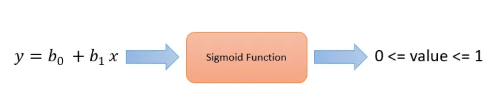
In the binary logistic model, We compute a linear combination of the inputs then, we pass it to sigmoid function that ensures 0≤𝜎(𝒙)≤1. Sigmoid function maps the linear combination of variables in value on to Bernoulli probability distribution with domain(0 to 1). This probability is further used for classification.
Logistic is a powerful classifier. Logistic regression is an appropriate algorithm when the output/dependent variable is binary/ have two values. For example, Yes-No, Positive-Negative etc. It can be used as
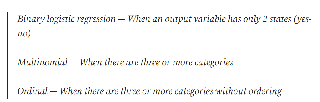
Binary logistic regression — When an output variable has only 2 states (yes-no)
Multinomial — When there are three or more categories
Ordinal — When there are three or more categories without ordering
In this blog, we will implement Binary logistic regression without using the built-in libraries for the algorithm.
What happens in Logistic Regression?
If you have studied linear regression you will know, in linear regression, we try to find the appropriate values of coefficient in a linear equation such that we get minimum root mean squared error (RMSE). Similarly, in logistic regression, we find the appropriate coefficient values in a linear equation which give the least classification error. We provide this linear equation to sigmoid function. The sigmoid function maps the entire data into real numbers of range 0 to 1. By setting threshold for this output we can easily classify the input data.
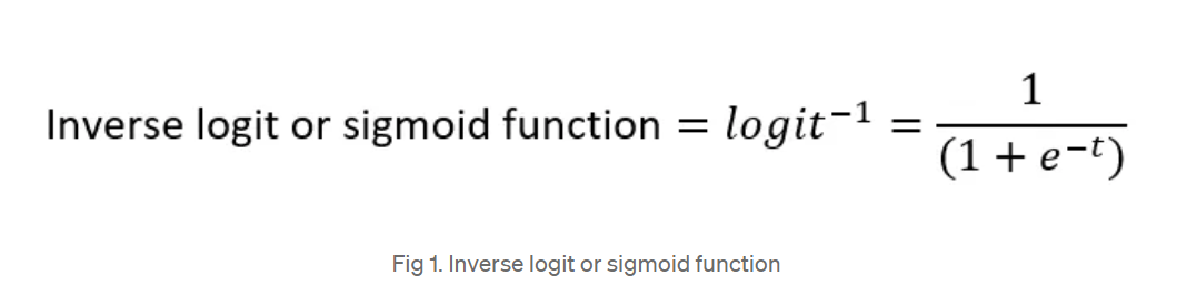 Where e is an Euler’s constant and t is the combination of variables. By using this we will receive a value between 0 and 1 for each input. Value above and below the threshold can be considered as different classes.
For better understanding, let’s assume t= b0+b1x, so we have to find appropriate values of b0 and b1 which gives better results. Thus, the sigmoid function for this equation will be,
For larger negative values, sigmoid function returns the values closer the zero and for larger positive values, sigmoid function returns the values closer the one .The graph obtained by this function is called s curve or logistic function curve.
Gradient descent is an optimization technique where we minimize the error by changing the values of coefficients repeatedly. To understand how logistic regression works, we will use gradient descent.
For this implementation, we are going to use the Breast cancer data set. By importing dataset module of sklearn library we can easily use this data set. It is a binary classification data set.
Now, let me run you through the implementation details — step by step.
First, we will import the numpy library for data manipulation. We will use dataset module of sklearn library to import data. Train Test Split module of sklearn library will be used for splitting the data into training and testing data. As well as we will use matplotlib for visualization.
Here is the github link to the implementation code in python.
We will store the independent variables in x and dependent/ output variable in y. Using train test split module of sklearn we will split our data.
The logistic sigmoid function is,
As I already mentioned, t is an equation consists of variables (Attributes) and coefficients. Our main aim is to find the coefficients of the equation in order to obtain good classification results.
Initially, we do not know the values of the coefficients. So, we will assign zero values for all weights and bias and small value for learning rate. Number of weights is equal to the number of independent variables. i.e. in the beginning, all coefficient value for the equation will be zero (b0, b1, …, bn =0).
As, values of all coefficient is 0 thus, Hence, Thus, irrespective of the value of x, we will receive 0.5 as an output, and we will get a straight line as s curve. We have defined a sigmoid function, where we can map our output into real numbers of range 0 to 1.
Now, we have to change the values for coefficients so, we can get a better model with a higher accuracy. After finding the better values we will create a linear model using those values. We will pass this model to sigmoid function which will give us the predicted value output variable. By defining a threshold, we can easily do the classification. Let’s assume, by using gradient descent we got new values for coefficients. Using these values we will create a model (An equation). We will pass this model to the sigmoid function to get predicted sigmoid values, which are between 0 and 1. By comparing these values to threshold we will perform the classification. To change the values of the coefficient, we will take derivative with respect to weights and bias to change the values of the coefficients. Then we will update the weights and bias by multiplying the negative learning rate to the derivatives we got w.r.t weights and bias.
Selecting range for for loop is an important choice you should do with this model. Bigger range for for loop will mean more number of iterations and may give better accuracy, but the time complexity will increase. In the other hand, smaller range may give poor fit as the final error achieved may not be near the point of minima. Also, using bigger range we might over-fit the model which results in less accuracy for test data. There are many stopping criteria for gradient descent like initializing the number of iteration and stop when change in prediction error is less than epsilon etc. I will try to explain detail gradient descent in another blog. Here we are defining the range for loop as stopping criteria.
Learning rate is a small value between 0 and 1 which controls the speed of change of weights. Bigger value of learning rate indicates rapid changes and fewer epochs but, it might skip the minima. After running the for loop, we will get some values of the coefficients and bias used in the model which will give better results.
This function will first create a linear model using new weights and bias. Then we will pass this model to sigmoid function which will return the y predicted values in the range of 0 to 1. We will set our threshold as 0.5. We will predict the label as 1 if the sigmoid function gives value greater than 0.5 else, we will predict it as 0. We will store these labels into y test predicted.
This model gives more than 92% accuracy with 1000 iterations. The accuracy of your model depends on many factors like threshold, Number of iteration, and type of data (right skewed, left skewed etc.). Different values of threshold or range for loop may give a better output. One way to find value of threshold and number of iterations is the Elbow method. I have plotted the number of iterations and the respective accuracy. We can select an elbow point from which accuracy decreases or stops changing significantly.
I have tried implementing this model using different values for number of iteration. I have received maximum accuracy i.e. 92.98% with 1000 iteration. For 2000 iteration, accuracy for model is 92.10%. Here, we can see the decrease in the accuracy even after increasing the number of iterations beyond 1000.
At 500 iterations, the accuracy obtained was ~91.23% . Hence depending on our accuracy goal, 500 iterations can also be a reasonable choice as a further increase by putting in twice the number of iterations only gives ~0.9% increase in accuracy.
Go Back To Home